Installing and Importing Dependencies

In [117]:
%pip install xgboost
Requirement already satisfied: xgboost in c:\users\geek\anaconda3\lib\site-packages (2.0.3)
Requirement already satisfied: numpy in c:\users\geek\anaconda3\lib\site-packages (from xgboost) (1.24.3)
Requirement already satisfied: scipy in c:\users\geek\anaconda3\lib\site-packages (from xgboost) (1.11.1)
Note: you may need to restart the kernel to use updated packages.
In [172]:
import math
import numpy as np
import pandas as pd
import matplotlib.pyplot as plt
import seaborn as sns
from pandas.plotting import scatter_matrix
from sklearn.preprocessing import OrdinalEncoder, StandardScaler, MinMaxScaler
from sklearn.base import BaseEstimator, TransformerMixin
from sklearn.model_selection import StratifiedShuffleSplit, RandomizedSearchCV, cross_val_score, GridSearchCV
from sklearn.impute import SimpleImputer
from sklearn.pipeline import Pipeline, FunctionTransformer
from sklearn.compose import ColumnTransformer
from sklearn.linear_model import LinearRegression
from sklearn.metrics import mean_squared_error
from sklearn.tree import DecisionTreeRegressor
from sklearn.neighbors import KNeighborsRegressor
import xgboost as xgb
from sklearn.ensemble import RandomForestRegressor
from scipy import stats
In [11]:
# smaller size plots
plt.rcParams.update({
    'font.size': 7,
    'figure.figsize': (4.3, 2.8),
    'lines.linewidth': 1,
})

0. Understanding Data

Diamond Cut

Because it is composed of a generally transparent material, diamond lets light pass through it, even in its most rough condition. But early on in history, stone cutters realized that you can get extra sparkle if you facet the diamond, and they set about finding out the best combination of facet size and shape and angle to get the most sparkle. Eventually, one design with 58 facets was shown to be the most efficient way to maximize the stone's best qualities and this became known as the ideal cut. It remains the industry standard, and is the shape that most people recognize as being a diamond shape.Read more..


Diamond Cut

Diamond Color

Color in diamonds comes from chemical impurities in the stone and imperfections in its molecular structure. The variety of impurities that can be found is large enough to give the stone a potential array of colors, the predominant ones being yellow and brown.Read more..

Diamond Color

Diamond Clarity

Clarity, as the name implies, refers to how clear the material is that the stone is made of, and what surface imperfections it may have. These have a direct effect on how light passes into a diamond and bounces around within it before finally exiting. Read more...

Diamond Clarity

Diamond Carat Weight

The size of the diamond is called its carat weight and actually refers to its mass. All other characteristics being equal, the carat weight is the biggest determinant of the price of a stone. Read more..

Diamond Carat Weight

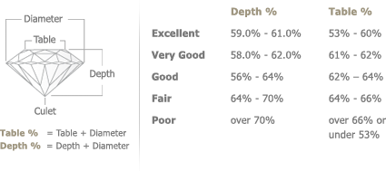
Diamond Depth Percentage

the deeper or heavier the gemstone and therefore the less sparkle and brilliance it exudes. The lower the depth percentage number, the shallower or glassier the diamond appears, also resulting in less sparkle and brilliance. Mathematicians have established the theoretical "ideal" depth percentage for a diamond to return maximum light and offer maximum brilliance.

Diamond Table Percentage

Table percentage is the length of the table facet divided by the diameter of the diamond. The higher the number, the bigger the table facet and the larger the surface area for leaking reflected light out of the diamond. The lower the number, the smaller the table dimensions and there is too little a surface area through which to see the internal brilliance of the diamond. As with the depth percentage, mathematicians have established the theoretical "ideal" table percentage for a diamond to offer maximum brilliance.

Read more..

Diamond Depth & Table Percentage

1. Reading & descovring Data

In [12]:
df = pd.read_csv('train.csv')
df.head()
Out[12]:
Id carat cut color clarity depth table price x y z
0 1 1.06 Ideal I SI2 61.8 57.0 4270 6.57 6.60 4.07
1 2 1.51 Premium G VVS2 60.9 58.0 15164 7.38 7.42 4.51
2 3 0.32 Ideal F VS2 61.3 56.0 828 4.43 4.41 2.71
3 4 0.53 Ideal G VS2 61.2 56.0 1577 5.19 5.22 3.19
4 5 0.70 Premium H VVS2 61.0 57.0 2596 5.76 5.72 3.50

the Id feature is just for indexing, it has no value for us, we shall drop it.

In [13]:
df.info()
<class 'pandas.core.frame.DataFrame'>
RangeIndex: 43152 entries, 0 to 43151
Data columns (total 11 columns):
 #   Column   Non-Null Count  Dtype  
---  ------   --------------  -----  
 0   Id       43152 non-null  int64  
 1   carat    43152 non-null  float64
 2   cut      43152 non-null  object 
 3   color    43152 non-null  object 
 4   clarity  43152 non-null  object 
 5   depth    43152 non-null  float64
 6   table    43152 non-null  float64
 7   price    43152 non-null  int64  
 8   x        43152 non-null  float64
 9   y        43152 non-null  float64
 10  z        43152 non-null  float64
dtypes: float64(6), int64(2), object(3)
memory usage: 3.6+ MB

No null was found

In [14]:
df.describe()
Out[14]:
Id carat depth table price x y z
count 43152.000000 43152.000000 43152.000000 43152.000000 43152.000000 43152.000000 43152.000000 43152.000000
mean 21576.500000 0.797855 61.747177 57.458347 3929.491912 5.731568 5.735018 3.538568
std 12457.053745 0.473594 1.435454 2.233904 3985.527795 1.121279 1.148809 0.708238
min 1.000000 0.200000 43.000000 43.000000 326.000000 0.000000 0.000000 0.000000
25% 10788.750000 0.400000 61.000000 56.000000 947.750000 4.710000 4.720000 2.910000
50% 21576.500000 0.700000 61.800000 57.000000 2401.000000 5.700000 5.710000 3.530000
75% 32364.250000 1.040000 62.500000 59.000000 5312.000000 6.540000 6.540000 4.040000
max 43152.000000 5.010000 79.000000 95.000000 18823.000000 10.740000 58.900000 31.800000

Dimension features (x,y,z) have a min of 0, that is not logical. we will handle this

2. Data visualization

Let's see some relations

In [20]:
correlation_matrix = df.corr(numeric_only=True)

plt.figure(figsize=(7, 4))
sns.heatmap(correlation_matrix, annot=True, cmap="coolwarm", fmt=".2f", linewidths=0.5)
plt.title('Correlation Matrix Heatmap')
plt.show()
  • At Carat bigger than around 4 is Fair cut, and at carat 5 it has it's max price
  • Most of data is concenrated around between 0.2 and 2.5 carat
  • the Ideal cut got it's highest price at around between 1 and 2.5 carat

Let's Look at the Categorical Data

In [15]:
ax = sns.countplot(x='cut', data=df)
for p in ax.patches:
    ax.annotate(f'{p.get_height()}', (p.get_x() + p.get_width() / 2., p.get_height()), ha='center', va='center', xytext=(0, 5), textcoords='offset points');
In [16]:
ax = sns.countplot(x='cut', data=df)
for p in ax.patches:
    ax.annotate(f'{p.get_height()}', (p.get_x() + p.get_width() / 2., p.get_height()), ha='center', va='center', xytext=(0, 5), textcoords='offset points');
In [17]:
ax = sns.countplot(x='clarity', data=df)
for p in ax.patches:
    ax.annotate(f'{p.get_height()}', (p.get_x() + p.get_width() / 2., p.get_height()), ha='center', va='center', xytext=(0, 5), textcoords='offset points');
In [22]:
sns.scatterplot(x='carat', y='price', data=df, hue='cut');
In [23]:
sns.scatterplot(x='depth', y='price', data=df, hue='cut');
  • High correlations exist between diamond price and attributes like carat and dimensions (x, y, z). These factors are closely related and likely influential in determining diamond prices.
  • Depth and Table have a weak negative correlation with each other.

3. Cleaning Data

Droping non-added value feature

In [24]:
df_no_id = df.drop("Id", axis=1)

Check for Duplicates

In [25]:
duplicates = df_no_id.duplicated()
num_duplicates = duplicates.sum()
num_duplicates
Out[25]:
97

There is a 97 Duplicate Rows, So we will remove them

In [29]:
df = df_no_id.drop_duplicates(keep='first')
df.duplicated().sum()
Out[29]:
0

Checking for Zero or Negative Values

In [30]:
numerics = ['int16', 'int32', 'int64', 'float16', 'float32', 'float64']
(df.select_dtypes(include=numerics)<=0).any(axis=1).sum()
Out[30]:
17
In [31]:
df.loc[(df.select_dtypes(include=numerics)<=0).any(axis=1)]
Out[31]:
carat cut color clarity depth table price x y z
571 1.10 Premium G SI2 63.0 59.0 3696 6.50 6.47 0.0
903 2.25 Premium I SI1 61.3 58.0 15397 8.52 8.42 0.0
1221 1.14 Fair G VS1 57.5 67.0 6381 0.00 0.00 0.0
4980 1.50 Good G I1 64.0 61.0 4731 7.15 7.04 0.0
6765 0.71 Good F SI2 64.1 60.0 2130 0.00 0.00 0.0
11221 2.80 Good G SI2 63.8 58.0 18788 8.90 8.85 0.0
13727 2.02 Premium H VS2 62.7 53.0 18207 8.02 7.95 0.0
14265 1.01 Premium F SI2 59.2 58.0 3837 6.50 6.47 0.0
16971 1.00 Premium G SI2 59.1 59.0 3142 6.55 6.48 0.0
21061 1.15 Ideal G VS2 59.2 56.0 5564 6.88 6.83 0.0
22171 1.00 Very Good H VS2 63.3 53.0 5139 0.00 0.00 0.0
24901 2.25 Premium H SI2 62.8 59.0 18034 0.00 0.00 0.0
27221 1.12 Premium G I1 60.4 59.0 2383 6.71 6.67 0.0
34065 1.01 Premium H I1 58.1 59.0 3167 6.66 6.60 0.0
35347 2.18 Premium H SI2 59.4 61.0 12631 8.49 8.45 0.0
39201 1.07 Ideal F SI2 61.6 56.0 4954 0.00 6.62 0.0
42898 2.20 Premium H SI1 61.2 59.0 17265 8.42 8.37 0.0

Zero values are not logical at dimensions columns, so we will drop those rows.

In [32]:
df = df[(df[['x','y','z']]!= 0).all(axis=1)]
print((df.select_dtypes(include=numerics)<=0).any(axis=1).sum())
df.shape
0
Out[32]:
(43038, 10)

Handling Outliers

In [33]:
fig, axs = plt.subplots(2,3,figsize=(14,6))
plt.subplots_adjust(hspace=0.4)
sns.scatterplot(data=df, x="price", y="carat", ax=axs[0][0]).set_title("carat");
sns.scatterplot(data=df, x="price", y="x", ax=axs[0][1]).set_title("x");
sns.scatterplot(data=df, x="price", y="y", ax=axs[0][2]).set_title("y");
sns.scatterplot(data=df, x="price", y="z", ax=axs[1][0]).set_title("z");
sns.scatterplot(data=df, x="price", y="table", ax=axs[1][1]).set_title("table");
sns.scatterplot(data=df, x="price", y="depth", ax=axs[1][2]).set_title("depth");
  • carat and x look's good to go.
  • for 'y' and 'z' I'll remove above 10.
  • for 'table' I'll remove above 80.
  • for 'depth' I'll remove below 50 or above 75.
In [34]:
outliers = df[
    (df.y > 10) | (df.z > 10) |\
    (df.table > 80) |\
    (df.depth < 50) | (df.depth > 75)]
df.drop(outliers.index, inplace=True)
print(f"Removed {outliers.shape[0]} Outliers")
Removed 11 Outliers
In [35]:
fig, axs = plt.subplots(2,3,figsize=(14,6))
plt.subplots_adjust(hspace=0.4)
sns.scatterplot(data=df, x="price", y="carat", ax=axs[0][0]).set_title("carat");
sns.scatterplot(data=df, x="price", y="x", ax=axs[0][1]).set_title("x");
sns.scatterplot(data=df, x="price", y="y", ax=axs[0][2]).set_title("y");
sns.scatterplot(data=df, x="price", y="z", ax=axs[1][0]).set_title("z");
sns.scatterplot(data=df, x="price", y="table", ax=axs[1][1]).set_title("table");
sns.scatterplot(data=df, x="price", y="depth", ax=axs[1][2]).set_title("depth");

Look's Good Except for 'z' may be removing below 2 also.

In [36]:
z_outliers = df[(df.z < 2)]
df.drop(z_outliers.index, inplace=True)
print(f"Removed {z_outliers.shape[0]} Outliers")
Removed 3 Outliers
In [37]:
sns.scatterplot(data=df, x="price", y="z").set_title("z");

Look's better now

4. Preparing Data

Feature Engineering

In [40]:
# Function to get the volume of Diamond more accurately
def volume_of_diamond(row):
    # Extracting length, width, and depth from the row
    length = row['x']
    width = row['y']
    depth = row['z']
    max_width=row['table']
    
    # Calculate the areas of the faces
    area_larger_face = length * max_width
    area_smaller_face = width ** 2
    
    
    # Calculate the volume
    volume = (1/3) * depth * (area_larger_face + area_smaller_face + math.sqrt(area_larger_face * area_smaller_face))
    
    return volume
In [72]:
#since (x y and z) can be replaced by the volume
processed_df = df.copy()
processed_df['volume'] = processed_df.apply(lambda x:(x["x"]*x["y"]*x["z"]), axis=1)
processed_df.drop(['x','y','z'], axis=1, inplace=True)
processed_df[:10]
Out[72]:
carat cut color clarity depth table price volume
0 1.06 Ideal I SI2 61.8 57.0 4270 176.483340
1 1.51 Premium G VVS2 60.9 58.0 15164 246.965796
2 0.32 Ideal F VS2 61.3 56.0 828 52.943373
3 0.53 Ideal G VS2 61.2 56.0 1577 86.422842
4 0.70 Premium H VVS2 61.0 57.0 2596 115.315200
5 0.90 Very Good G IF 63.1 58.0 5670 145.652094
6 0.71 Very Good F VS1 61.8 60.0 3017 113.239620
7 0.70 Ideal F SI1 61.3 57.0 2288 116.175488
8 0.59 Ideal D VS1 60.9 56.0 2175 96.761280
9 0.31 Very Good G VVS1 59.8 62.0 761 50.260770
In [42]:
processed_df.hist(figsize=(8, 8));
In [43]:
sns.scatterplot(x='volume', y='price', data=processed_df, hue='cut');
In [44]:
attributes = ["price", "carat", "depth", "table", "volume"]
scatter_matrix(processed_df[attributes], figsize=(8.4,6), s=20);

Ordinal Encoding

We need to give the categorical data numerical values

In [73]:
enc_processed_df = processed_df.copy()

# Ordering each category
colors_cats = ['J', 'I', 'H', 'G', 'F', 'E', 'D']
cuts_cats = ['Fair', 'Good', 'Very Good', 'Premium', 'Ideal']
clarities_cats = ['I1', 'SI2', 'SI1', 'VS2', 'VS1', 'VVS2', 'VVS1', 'IF']

# Transform ordinal columns
ord_enc = OrdinalEncoder(categories=[colors_cats, cuts_cats, clarities_cats])
diamond_cats_encoded = ord_enc.fit_transform(enc_processed_df[['color', 'cut', 'clarity']])

enc_processed_df[['color','cut','clarity']] = diamond_cats_encoded
enc_processed_df.head()
Out[73]:
carat cut color clarity depth table price volume
0 1.06 4.0 1.0 1.0 61.8 57.0 4270 176.483340
1 1.51 3.0 3.0 5.0 60.9 58.0 15164 246.965796
2 0.32 4.0 4.0 3.0 61.3 56.0 828 52.943373
3 0.53 4.0 3.0 3.0 61.2 56.0 1577 86.422842
4 0.70 3.0 2.0 5.0 61.0 57.0 2596 115.315200
In [74]:
enc_processed_df.corr().price.sort_values(ascending=False)
Out[74]:
price      1.000000
volume     0.924212
carat      0.922247
table      0.127605
depth     -0.013130
cut       -0.055436
clarity   -0.146704
color     -0.170819
Name: price, dtype: float64
In [75]:
enc_processed_df.head()
Out[75]:
carat cut color clarity depth table price volume
0 1.06 4.0 1.0 1.0 61.8 57.0 4270 176.483340
1 1.51 3.0 3.0 5.0 60.9 58.0 15164 246.965796
2 0.32 4.0 4.0 3.0 61.3 56.0 828 52.943373
3 0.53 4.0 3.0 3.0 61.2 56.0 1577 86.422842
4 0.70 3.0 2.0 5.0 61.0 57.0 2596 115.315200
In [76]:
enc_processed_df.describe()
Out[76]:
carat cut color clarity depth table price volume
count 43024.000000 43024.000000 43024.000000 43024.000000 43024.000000 43024.000000 43024.000000 43024.000000
mean 0.797207 2.905099 3.406634 3.046369 61.747197 57.458509 3927.054737 129.739793
std 0.472207 1.114481 1.701998 1.649016 1.421744 2.225115 3981.731726 76.225777
min 0.200000 0.000000 0.000000 0.000000 50.800000 43.000000 326.000000 31.707984
25% 0.400000 2.000000 2.000000 2.000000 61.000000 56.000000 947.000000 65.189759
50% 0.700000 3.000000 3.000000 3.000000 61.800000 57.000000 2401.000000 114.852720
75% 1.040000 4.000000 5.000000 4.000000 62.500000 59.000000 5311.000000 170.822400
max 4.130000 4.000000 6.000000 7.000000 72.200000 79.000000 18823.000000 633.355000
In [77]:
plt.figure(figsize=(8,5))
sns.heatmap(enc_processed_df.corr(), annot=True, linewidths=0.5, cmap="coolwarm")
plt.title('Correlation Heatmap')
plt.show()

Surprisingly the clarity, color, and cut have a negative or no correlation with price, but this is because the Diamond carat (weight) and volume have more influence on the price.

5. Preparing model

In [78]:
# getting columns index for numeric features after dropping categorical features
x_ix2, y_ix2, z_ix2 = [
    list(df.drop(["cut", "color", "clarity", "price"], axis=1).columns).index(col)
    for col in ("x", "y", "z")]
class VolumeAttributesAdder(BaseEstimator, TransformerMixin):
    """Combine Attributes"""
    def __init__(self):
        pass
    def fit(self, X, y=None):
        return self
    def transform(self, X, y=None):
        # Calculate the volume
        volume = X[:, x_ix2] * X[:, y_ix2] * X[:, z_ix2]
        
        # Drop x', 'y', and 'z' columns
        X = np.delete(X, [x_ix2, y_ix2, z_ix2], axis=1)
        
        return np.c_[X, volume]

Spliting Data to Train and Test Sets

Using carat features distribution we will make a stratified split to get fairly similar train and test sets.

In [81]:
df.loc[:, "carat_cat"] = pd.cut(df["carat"],
                               bins=[0.19, 0.5, 0.75, 1, 1.5, np.inf],
                               labels=[1, 2, 3, 4, 5])
df["carat_cat"].hist();
In [82]:
split = StratifiedShuffleSplit(n_splits=10, test_size=0.2, random_state=42)

for train_index, test_index in split.split(df, df["carat_cat"]):
    train_set = df.iloc[train_index]
    test_set = df.iloc[test_index]
In [83]:
# Checking Sets Smilarity after Splitting

original_ratios = df["carat_cat"].value_counts() / len(df)
train_ratios = train_set["carat_cat"].value_counts() / len(train_set)
test_ratios = test_set["carat_cat"].value_counts() / len(test_set)
print(list(zip(original_ratios,train_ratios,test_ratios)))
[(0.35075771662328004, 0.3507655655306662, 0.35072632190586867), (0.22401450353291186, 0.22400418373572736, 0.2240557815223707), (0.21139364075864633, 0.2113948691129899, 0.2113887274840209), (0.11307642246188174, 0.11307707952003254, 0.11307379430563626), (0.10075771662328004, 0.10075830210058398, 0.10075537478210343)]
In [84]:
df= df.drop('carat_cat',axis=1)
train_set = train_set.drop('carat_cat',axis=1)
test_set = test_set.drop('carat_cat',axis=1);

Looks Good 👍

Creating Pipelines

In [85]:
# dropping the target feature from sets

x_train= train_set.drop('price',axis=1)
y_train= train_set['price']
x_test= test_set.drop('price',axis=1)
y_test= test_set['price']
In [86]:
num_attribs = ["carat", "depth", "table", "x", "y", "z"]
cat_attribs = ['color', 'cut', 'clarity']

num_pipeline = Pipeline([
    ('imputer', SimpleImputer(strategy="median")),
    ('attribs_adder', VolumeAttributesAdder()),
    ('std_scaler', StandardScaler()),
])

cat_pipeline=Pipeline([
        ('imputer',SimpleImputer(strategy='most_frequent')),
        ('ordinalencode',OrdinalEncoder(categories=[colors_cats, cuts_cats, clarities_cats])),
        ('scaler',StandardScaler())
])

full_pipeline = ColumnTransformer([
    ("norm_num", num_pipeline, num_attribs),
    ("cat", cat_pipeline, cat_attribs)
])

x_train_prepared = full_pipeline.fit_transform(x_train)
x_test_prepared = full_pipeline.fit_transform(x_test)
In [102]:
x_train_prepared.shape
Out[102]:
(34419, 7)

Models Creation

Linear Regression Model

In [88]:
linear_model=LinearRegression()
linear_model.fit(x_train_prepared,y_train)
Out[88]:
LinearRegression()
In a Jupyter environment, please rerun this cell to show the HTML representation or trust the notebook.
On GitHub, the HTML representation is unable to render, please try loading this page with nbviewer.org.
LinearRegression()

Evaluating Linear Regression Model

In [154]:
linear_model_score = linear_model.score(x_test_prepared, y_test)
linear_model_score
Out[154]:
0.9121912840790678
In [90]:
lin_predic = linear_model.predict(x_test_prepared)
lin_rmse = mean_squared_error(
    y_test,
    lin_predic,
    squared=False  #RMSE
)
lin_rmse
Out[90]:
1187.7526647447082
In [91]:
lin_scores = cross_val_score(
  linear_model,
  x_test_prepared,
  y_test,
  scoring ="neg_mean_squared_error",
  cv = 10
)
lin_rmse_scores = np.sqrt(-lin_scores)
print("Scores: ", lin_rmse_scores)
print("Mean: ", lin_rmse_scores.mean())
print("Standard Deviation: ", lin_rmse_scores.std())
Scores:  [1174.83347894 1223.31110693 1249.26628419 1084.4072613  1156.50396718
 1190.38882453 1197.95744941 1218.23196731 1181.05380673 1187.45414077]
Mean:  1186.340828730001
Standard Deviation:  42.35220527895303

Decision Tree Regressorion Model

In [92]:
tree_model=DecisionTreeRegressor(random_state = 42)
tree_model.fit(x_train_prepared,y_train)
Out[92]:
DecisionTreeRegressor(random_state=42)
In a Jupyter environment, please rerun this cell to show the HTML representation or trust the notebook.
On GitHub, the HTML representation is unable to render, please try loading this page with nbviewer.org.
DecisionTreeRegressor(random_state=42)

Evaluating Decision Tree Regressorion Model

In [155]:
tree_model_score = tree_model.score(x_test_prepared, y_test)
tree_model_score
Out[155]:
0.9679069119401801
In [94]:
tree_predic = tree_model.predict(x_test_prepared)
tree_rmse = mean_squared_error(
    y_test,
    tree_predic,
    squared=False
)
tree_rmse
Out[94]:
718.0636696439942
In [95]:
tree_scores = cross_val_score(
  tree_model,
  x_test_prepared,
  y_test,
  scoring ="neg_mean_squared_error",
  cv = 10
)
tree_rmse_scores = np.sqrt(-tree_scores)
print("Scores: ", tree_rmse_scores)
print("Mean: ", tree_rmse_scores.mean())
print("Standard Deviation: ", tree_rmse_scores.std())
Scores:  [801.20055985 738.07947391 743.45806708 777.63607788 866.47596781
 730.69331822 806.99245209 901.34929476 860.48244665 757.15929939]
Mean:  798.3526957643631
Standard Deviation:  57.04567321384389

K Nearest Neighbor Regression Model

In [110]:
knns = []
for k in range(1, 20):
    knn_regressor = KNeighborsRegressor(n_neighbors=k)
    knn_regressor.fit(x_train_prepared, y_train)
    knns.append((k, knn_regressor.score(x_test_prepared, y_test)))
best_knn_values = max(knns, key = lambda i : i[1])
print(f'Score for best k={best_knn_values[0]}: is {best_knn_values[1]}')
Score for best k=10: is 0.9674622198337178
In [111]:
knn_model = KNeighborsRegressor(n_neighbors=10)
knn_model.fit(x_train_prepared, y_train)
Out[111]:
KNeighborsRegressor(n_neighbors=10)
In a Jupyter environment, please rerun this cell to show the HTML representation or trust the notebook.
On GitHub, the HTML representation is unable to render, please try loading this page with nbviewer.org.
KNeighborsRegressor(n_neighbors=10)

Evaluating K Nearest Neighbor Regression Model

In [156]:
knn_model_score = knn_model.score(x_test_prepared, y_test)
knn_model_score
Out[156]:
0.9674622198337178
In [113]:
knn_predic = knn_model.predict(x_test_prepared)
knn_rmse = mean_squared_error(
    y_test,
    knn_predic,
    squared=False
)
knn_rmse
Out[113]:
723.0214147901888
In [114]:
knn_scores = cross_val_score(
  knn_model,
  x_test_prepared,
  y_test,
  scoring ="neg_mean_squared_error",
  cv = 10
)
knn_rmse_scores = np.sqrt(-knn_scores)
print("Scores: ", knn_rmse_scores)
print("Mean: ", knn_rmse_scores.mean())
print("Standard Deviation: ", knn_rmse_scores.std())
Scores:  [798.19424497 839.90636493 885.33098311 712.5232469  827.62281422
 735.84170983 860.69248202 817.72519963 949.42519402 837.546358  ]
Mean:  826.480859763202
Standard Deviation:  64.90890704051506

XGBoost Model

In [138]:
xgb_model = xgb.XGBRegressor(n_estimators=100, objective='reg:squarederror', tree_method='hist', eta=0.1, max_depth=3, random_state=42)
xgb_model.fit(x_train_prepared, y_train)
Out[138]:
XGBRegressor(base_score=None, booster=None, callbacks=None,
             colsample_bylevel=None, colsample_bynode=None,
             colsample_bytree=None, device=None, early_stopping_rounds=None,
             enable_categorical=False, eta=0.1, eval_metric=None,
             feature_types=None, gamma=None, grow_policy=None,
             importance_type=None, interaction_constraints=None,
             learning_rate=None, max_bin=None, max_cat_threshold=None,
             max_cat_to_onehot=None, max_delta_step=None, max_depth=3,
             max_leaves=None, min_child_weight=None, missing=nan,
             monotone_constraints=None, multi_strategy=None, n_estimators=100,
             n_jobs=None, num_parallel_tree=None, ...)
In a Jupyter environment, please rerun this cell to show the HTML representation or trust the notebook.
On GitHub, the HTML representation is unable to render, please try loading this page with nbviewer.org.
XGBRegressor(base_score=None, booster=None, callbacks=None,
             colsample_bylevel=None, colsample_bynode=None,
             colsample_bytree=None, device=None, early_stopping_rounds=None,
             enable_categorical=False, eta=0.1, eval_metric=None,
             feature_types=None, gamma=None, grow_policy=None,
             importance_type=None, interaction_constraints=None,
             learning_rate=None, max_bin=None, max_cat_threshold=None,
             max_cat_to_onehot=None, max_delta_step=None, max_depth=3,
             max_leaves=None, min_child_weight=None, missing=nan,
             monotone_constraints=None, multi_strategy=None, n_estimators=100,
             n_jobs=None, num_parallel_tree=None, ...)

Evaluating XGBoost Model

In [157]:
xgb_model_score = xgb_model.score(x_test_prepared, y_test)
xgb_model_score
Out[157]:
0.8702517721291727
In [140]:
xgb_predic = xgb_model.predict(x_test_prepared)
xgb_rmse = mean_squared_error(
    y_test,
    xgb_predic,
    squared=False
)
xgb_rmse
Out[140]:
1443.8029264452205
In [141]:
xgb_scores = cross_val_score(
  xgb_model,
  x_test_prepared,
  y_test,
  scoring ="neg_mean_squared_error",
  cv = 10
)
xgb_rmse_scores = np.sqrt(-xgb_scores)
print("Scores: ", xgb_rmse_scores)
print("Mean: ", xgb_rmse_scores.mean())
print("Standard Deviation: ", xgb_rmse_scores.std())
Scores:  [615.77477368 623.35241735 633.37886736 588.17990089 603.28828395
 562.28857428 637.4057718  688.28302082 670.27485766 597.12049001]
Mean:  621.9346957807678
Standard Deviation:  35.790541749356045

Random Forest Model

In [150]:
forest_model = RandomForestRegressor(n_estimators=100, random_state=42)
forest_model.fit(x_train_prepared, y_train)
Out[150]:
RandomForestRegressor(random_state=42)
In a Jupyter environment, please rerun this cell to show the HTML representation or trust the notebook.
On GitHub, the HTML representation is unable to render, please try loading this page with nbviewer.org.
RandomForestRegressor(random_state=42)

Evaluating Random Forest Model

In [158]:
forest_model_score = forest_model.score(x_test_prepared, y_test)
forest_model_score
Out[158]:
0.9816880900862357
In [152]:
forest_predic = forest_model.predict(x_test_prepared)
forest_rmse = mean_squared_error(
    y_test,
    forest_predic,
    squared=False
)
forest_rmse
Out[152]:
542.4054216291132
In [153]:
forest_scores = cross_val_score(
  forest_model,
  x_test_prepared,
  y_test,
  scoring ="neg_mean_squared_error",
  cv = 10
)
forest_rmse_scores = np.sqrt(-forest_scores)
print("Scores: ", forest_rmse_scores)
print("Mean: ", forest_rmse_scores.mean())
print("Standard Deviation: ", forest_rmse_scores.std())
Scores:  [611.73659639 554.55174792 588.78002293 602.7504877  593.06243663
 492.50670738 601.43544067 691.99361443 621.67443942 560.22958046]
Mean:  591.8721073926545
Standard Deviation:  48.78053804811605

Comparing Models

In [162]:
data = [
    ['Linear Regression', linear_model_score, lin_rmse, lin_rmse_scores.mean()],
    ['Decision Tree', tree_model_score, tree_rmse, tree_rmse_scores.mean()],
    ['K Nearest Neighbor', knn_model_score, knn_rmse, knn_rmse_scores.mean()],
    ['XGBoost', xgb_model_score, xgb_rmse, xgb_rmse_scores.mean()],
    ['Random Forest', forest_model_score, forest_rmse, forest_rmse_scores.mean()],
]
df = pd.DataFrame(data, columns=['Model', 'Score', "RMSE", "CV_Mean"])
df
Out[162]:
Model Score RMSE CV_Mean
0 Linear Regression 0.912191 1187.752665 1186.340829
1 Decision Tree 0.967907 718.063670 798.352696
2 K Nearest Neighbor 0.967462 723.021415 826.480860
3 XGBoost 0.870252 1443.802926 621.934696
4 Random Forest 0.981688 542.405422 591.872107

From the Comparison, we can see that the Random Forest Model is the best candidate.

6- Fine-Tuning the Model

Finding better parameters values using Grid Search CV

In [173]:
# Define the parameter grid
param_grid = {
    'n_estimators': [100, 200, 300],
    'max_features': [3, 5, 7]
}

# Initialize the GridSearchCV
grid_search = GridSearchCV(estimator=RandomForestRegressor(random_state=42),
                           param_grid=param_grid,
                           cv=5,
                           n_jobs=-1,
                           verbose=2)

# Fit the model
grid_search.fit(x_train_prepared, y_train)
Fitting 5 folds for each of 9 candidates, totalling 45 fits
Out[173]:
GridSearchCV(cv=5, estimator=RandomForestRegressor(random_state=42), n_jobs=-1,
             param_grid={'max_features': [3, 5, 7],
                         'n_estimators': [100, 200, 300]},
             verbose=2)
In a Jupyter environment, please rerun this cell to show the HTML representation or trust the notebook.
On GitHub, the HTML representation is unable to render, please try loading this page with nbviewer.org.
GridSearchCV(cv=5, estimator=RandomForestRegressor(random_state=42), n_jobs=-1,
             param_grid={'max_features': [3, 5, 7],
                         'n_estimators': [100, 200, 300]},
             verbose=2)
RandomForestRegressor(random_state=42)

Evalute Final Model

In [177]:
grid_cvres = grid_search.cv_results_

# Inspect mean_test_score before taking the square root
for mean_score, params in zip(grid_cvres["mean_test_score"], grid_cvres["params"]):
    if mean_score < 0:
        rmse = np.sqrt(-mean_score)
    else:
        rmse = np.sqrt(mean_score)
    
    # Print the RMSE and parameters, handling invalid sqrt values
    if np.isnan(rmse):
        print("Invalid RMSE encountered for parameters:", params)
    else:
        print(rmse, params)
0.9902484383256457 {'max_features': 3, 'n_estimators': 100}
0.9902644555189066 {'max_features': 3, 'n_estimators': 200}
0.9902586157222898 {'max_features': 3, 'n_estimators': 300}
0.9900592995110594 {'max_features': 5, 'n_estimators': 100}
0.9901505064301226 {'max_features': 5, 'n_estimators': 200}
0.9901705220269647 {'max_features': 5, 'n_estimators': 300}
0.989890323588074 {'max_features': 7, 'n_estimators': 100}
0.989941756271822 {'max_features': 7, 'n_estimators': 200}
0.9899542412322111 {'max_features': 7, 'n_estimators': 300}
In [178]:
final_grid_model = grid_search.best_estimator_
final_grid_model
Out[178]:
RandomForestRegressor(max_features=3, n_estimators=200, random_state=42)
In a Jupyter environment, please rerun this cell to show the HTML representation or trust the notebook.
On GitHub, the HTML representation is unable to render, please try loading this page with nbviewer.org.
RandomForestRegressor(max_features=3, n_estimators=200, random_state=42)
In [179]:
# final_predictions = final_model.predict(x_test_prepared)
final_grid_predictions = final_grid_model.predict(x_test_prepared)


# final_mse = mean_squared_error(y_test, final_predictions)
final_grid_mse = mean_squared_error(y_test, final_grid_predictions)
final_grid_rmse = np.sqrt(final_grid_mse)
final_grid_rmse
Out[179]:
531.0001671494201
In [180]:
confidence = 0.95
squared_errors = (final_grid_predictions - y_test) ** 2
np.sqrt(stats.t.interval(confidence, len(squared_errors) - 1,
                         loc=squared_errors.mean(),
                         scale=stats.sem(squared_errors)))
Out[180]:
array([506.71441965, 554.22274578])

Finally, we have a Model which can make predictions with confidence levels (506.7 to 554.2).

Thanks for Reading to the End 🥰